본 포스팅에서는 GAN(Generative Adversarial Network)를 이용한 Anomaly Detection(이상치 탐지)에 대해서 어떤 알고리즘들이 제안되었는지를 알아본다.

1. AnoGAN

AnoGAN은 GAN을 이용한 anomaly detection의 가장 시초격 논문이다. 이 논문은 다음과 같은 문제 세팅을 하고 있다.

• $M$개의 정상 이미지들. 각각은 $I_m$으로서, $m=1,\cdots, M$이다.
• $I_m\in\mathbb{R}^{a\times b}$ 즉, 이미지들은 $a\times b$사이즈이다.
• 각 이미지 $I_m$에 때해서, 우리는 $K$개의 2차원 패치 $x_{k,m}\in\mathcal{X}$를 뜯는다. 이 때 $k=1,\cdots, K$이다.
• 학습 동안에, 우리는 $\langle I_m\rangle$이미지들만 GAN에게 보여준다. 즉, 정상 데이터에 대한 manifold를 학습시킨다.
• 테스트 동안에, 우리는 $(y_n, l_n)$으로 이루어진 쌍을 AnoGAN에게 보여주는데, 이 때 $y_n$은 학습 동안에 보지 못한 데이터이고, $l_n$은 0 혹은 1로서 정답 레이블이다.

이렇게 problem formulation을 해놓고 나서 제대로 된 학습과 테스트 과정을 기술한다.

• Generator은 latent space $\mathcal{Z}$의 원소 $z$로부터 이미지를 생성해내는 함수 $G:z\mapsto x$를 배운다.
• 하지만, 일반적으로 이 $G$의 역함수 $\mu : x\mapsto z$는 존재하지 않는다.
• 따라서, 저자들이 원하는 것은 최적의 latent vector $z_{\Gamma}$를 찾아서 주어진 이미지와 가장 유사한 정상 이미지를 만드는 것이다.

구체적인 anomaly detection 과정은 다음과 같다.

1. Latent space $\mathcal{Z}$에서 랜덤하게 샘플 $z_1$을 뽑는다.
2. loss $\mathcal{L}$을 최소화하는 방향으로 $z_{\gamma}$, $\gamma = 1,\cdots,\Gamma$를 업데이트한다.

3. loss는 두 항으로 이루어져 있는데, Residual loss와 Discriminator loss가 바로 그것이다.
   3-1. Residual loss $\mathcal{L}_{R}(z_{\gamma}) = \sum |x - G(z_{\gamma})|$. 3-2. Discriminator loss $\mathcal{L}_D(z_{\gamma}) = \sum |f(x) - f(G(z_{\gamma}))|$ (단, $f$는 discriminator의 중간 단계의 output)

4. Total loss $\mathcal{L}(z_{\gamma}) = (1-\lambda)\cdot L_{R}(z_{\gamma}) + \lambda\cdot L_{D}(z_{\gamma})$

그리고는 Anomaly score을 구한다.

\[A(x) = (1-\lambda)\cdot R(x) + \lambda\cdot D(x)\]

이 때 residual score $R(x)$와 discriminator score $D(x)$는 latent space $\mathcal{Z}$에서 마지막 업데이트가 된 후의 값이다.

2. EGBAD(Efficient GAN based Anomlay Detection)

EGBAD는 BiGAN의 아이디어를 차용한다. 즉, 학습 과정에서 generator $G$, discriminator $D$, encoder $E$를 모두 학습한다.

이 때 푸는 optimization problem은 다음과 같다:

\[V(D,E,G) = \mathbb{E}\_{x\sim p_X}\bigg(\mathbb{E}\_{z\sim p_{E}(\cdot|x)}\bigg(\log D(x,z)\bigg)\bigg)+\mathbb{E}\_{z\sim p_Z}\bigg(\mathbb{E}\_{x\sim p_G(\cdot|z)}\bigg(1-\log D(x,z)\bigg)\bigg)\]

이 때

• $p_X(x)$ : data의 distribution
• $p_Z(z)$ : lateent representation의 distribution
• $p_E(z\mid x)$, $p_G(x\mid z)$ : encoder와 generator로부터 유도된 distribution

$G, D$, 그리고 $E$를 훈련시킨 다음, 우리는 AnoGAN과 유사한 score function $A(x)$를 정의한다:

\[A(x) = \alpha L_{G}(x) + (1-\alpha) L_D(x)\]

이 때

• $L_G(x) =

  x - G(E(x))

  _1$

• $L_D(x)$는 두 가지 방법으로 정의할 수 있다.
  – $L_D(x) = \sigma(D(x,E(x)),1)$, 이 때 $\sigma$는 sigmoid cross-entropy loss이다.
  – $L_D(x) = |f_D(x,E(x)) - f_D(G(E(x)),E(x))|_1$

3. GANomaly

GANomaly는 다음과 같은 구조를 가지고 있다.

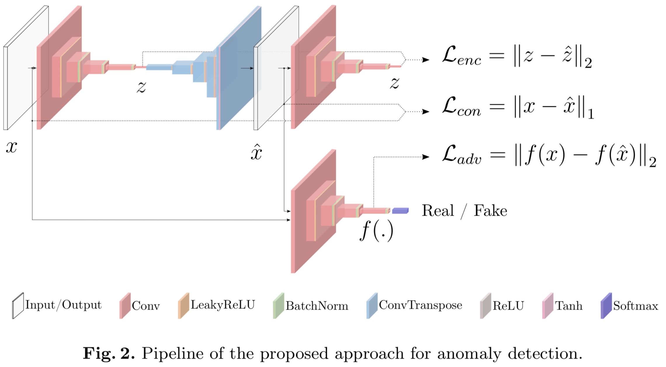
이를 설명하면 다음과 같다.

1. Bow-tie autoencoder network : Generator $G$는 input image $x$를 인풋으로 받아서 $G_E$를 forward-pass encoder에 통과시킨다. 이렇게 통과시킨 output을 $z\in\mathbb{R}^d$라고 하고, generator network $G$의 decoder $G_D$는 $z$를 새로운 이미지 $\hat{x}$로 reconstruct 시킨다. 즉, $\hat{x} = G_D(G_E(x))$이다.

2. Encoder Network $E$ : $G$에 의해 reconstruct된 이미지 $\hat{x}$를 압ㅊ축시킨다. 이것은 $G_E$와 parametrizaion만 다르고 구조는 같은 네트워크이다. $E$는 $\hat{x}$를 새로운 latent vector $\hat{z}$로 encode시킨다. 이 $\hat{z}$또한 $\mathbb{R}^d$의 원소이다.

3. Discriminator network $D$ : $x$와 $\hat{x}$가 진짜인지 가짜인지를 구분한다. DCGAN과 같은 구조를 가지고 있다.

그리고 나면 모델 훈련은 다음과 같은 세 loss를 최소화하는 과정으로 이루어진다.

\[\mathcal{L}\_{adv} = \mathbb{E}\_{x\sim p_X}||f(x) - \mathbb{E}\_{x\sim p_X} f(G(x))||\_2\] \[\mathcal{L}\_{con} = \mathbb{E}\_{x\sim p_X}||x - G(x)||\_2\] \[\mathcal{L}\_{enc} = \mathbb{E}\_{x\sim p_X} ||G_E(x) - E(G(x))||\_2\]

이들의 linear combination $\mathcal{L}$을 total loss로서 정의한다.

\[\mathcal{L} = w_{adv}\mathcal{L}\_{adv} + w_{con}\mathcal{L}\_{con} + w_{enc}\mathcal{L}\_{enc}\]

이 때 $G$는 generator이고, $f$는 discriminator $D$의 intermediate output이고, $E$는 encoder이다.

이렇게 학습이 완료된 다음에는 anomaly score를 정의하여 testing을 하는데, 그 과정은 다음과 같다.

\[\mathcal{A}(\hat{x}) = ||G_E(\hat{x}) - E(G(\hat{x}))||\_1\]

이렇게 모든 이미지에 대해서 anomaly score를 계산한 다음, 이들을 다 모은 집합 $\mathcal{S}$를 normalize한다:

\[s\_i' = \frac{s_i - \min\mathcal{S}}{\max\mathcal{S} - \min\mathcal{S}}\]