Optimal Transport driven CycleGAN for Unsupervised Learning in Inverse Problems

What is Inverse Problem?

Introduction to Inverse Problem in Imaging - Book

The CT-computer-generated imaged provided the first example of images obtained by solving a mathematical problem which belong to the class of the so-called inverse and ill-posed problems.

What is an inverse problem?

J.B.Keller : “We call two problems inverse of one another if the formulation of each involves all or part of the solution of the other.

• Direct problem : One of two problems has been studied extensively for some time. It is a problem oriented along a cause-effect sequence
  • Heat propagation (one-dimensional) given the initial and boundary condition $u(x,0) = f(x)$; $u(0,t) = u(a,t) = 0$
  \[\frac{\partial^2 u}{\partial x^2} = \frac{1}{D}\frac{\partial u}{\partial t}\]
  • Solution of the heat equation with utilizing Fourier transform is given by
  \[u(x,t) = \sum_{n=1}^{\infty}f_n e^{-D(\pi n/a)^2t}\sin(\pi n\frac{x}{a})\]
  • where
  \[f_n = \frac{2}{a}\int_{0}^a f(x)\sin(\pi n\frac{x}{a})dx\]
  • Since Fourier coefficients $f_n$ tend to zero when $n\to\infty$, it follows that only a finite number of Fourier coefficients, let us say $N_{\varepsilon}$ is known. $\to$ Direct problem
  • We conclude that the information content of the solution is much smaller than the information content of the data
• Inverse problem : The other has never been studied and is not so well understood.
  • Inverse problem for the heat equation: Determining the temperature distribution at $t=0$, being given the temperature distribution at the time $t=T>0$.
  • Therefore, the data function is now given by $u(x,T)$, while the unknown function is $f(x)$.
  • This is ill-posed problem.

What is the ill-posed problem?

• Well-posed problem: Introduced by French mathematician Jacques Hadamard in a paper published in 1902 on boundary value problems for PDE and their physical interpretation.
• A problem is well-posed if when its solution is unique and exists for arbitrary data.
• Example of well-posed problem by the initial value problem, also called the Cauchy problem, for the D’Alembert equation which is basic in the description of wave propagation

\[\frac{\partial^2 u}{\partial x^2} - \frac{1}{c}\frac{\partial^2 u}{\partial t^2}\]

• where $c$ is the wave velocity. If we consider the following initial condition data at $t=0$; $u(x,0) = f(x)$, $\displaystyle\frac{\partial u}{\partial t}(x,0)=0$, then there exists a unique solution given by

\[u(x,t) = \frac{1}{2}[f(x-ct)+f(x+ct)]\]

• for any continuous function $f(x)$

• Example of ill-posed problem is also given by Hadamard, is the Cauchy problem of the Laplace equation in two variables

\[\frac{\partial^2u}{\partial x^2}+\frac{\partial^2u}{\partial y^2}=0\]

• If we consider the following Cauchy data at $y=0$, given by $u(x,0) = \frac{1}{n}\cos(nx)$, $\displaystyle\frac{\partial u}{\partial y}(x,0)=0$, then there is an unique solution of Laplace equation given by

\[u(x,y) = \frac{1}{n}\cos(nx)\cosh(ny)\]

• It is possible to show that the solution does not exist for arbitrary data but only for data with some specific mathematical property.
• It is known now that the basic inverse problem of electrocardiography, i.e., the reconstruction of the epicardial potential from body surface maps, can be formulated just as a Cauchy problem for an elliptic equation, i.e., a generalization of the Laplace equation.

Summarize

• A directed problem, i.e., a problem oriented along a cause-effect sequence, is well-posed while the corresponding inverse problem, which implies a reversal of the cause-effect sequence is ill-posed.

Inverse problem in images

• First, defined the class of the objects to be images, which will be described by suitable functions with certain properties.
• In this class, we also need a distance, in order to establish when two objects are close and when they are not.

• We denote this space $\mathcal{X}$ and we will call it object space.

• Second, to solve the direct problem, i.e., to compute, for each object, the corresponding image which can be called the computed image or the noise-free image.
• Since the direct problem is well-posed, to each object we associate one, and only one, image.
• As we already remarked, this image may be rather smooth as a consequence of the fact that its information content is smaller than the information content of the corresponding object.

• This property of smoothness, however, may not be true for the measured images, also called noisy images, because they correspond to some noise-free image corrupted by the noise affecting the measurement process.

• Third, define the class of the images in such a way that it contains both the noise-free and the noisy images. It is convenient to introduce a distance also in this class. We denote corresponding function space by $\mathcal{Y}$ and we will call it the image space.

• In conclusion, the solution of the direct problem defines a mapping(operator), denoted by $A$, which transforms any object of the space $\mathcal{X}$ into a noise-free image of the space $\mathcal{Y}$. This operator is continuous, i.e., the images of two close objects are also close, because the direct problem is well-posed.
• The set of the noise-free images usually called, in mathematics, the range of the operator $A$, and as follows from our previous remark, this range does not coincide with the image space $\mathcal{Y}$ because this space contains also the noisy images.

Introduction

• In inverse problems, a noisy measurement $y\in\mathcal{Y}$ from an unobserved image $x\in\mathcal{X}$ is modeled by

\[y=\mathcal{H}x+w\]

• where $w$ is the noise, and $\mathcal{H}:\mathcal{X}\to\mathcal{Y}$ is the measurement operator. In inverse problems, the measurement operator is usually represented by an integral equation:

\[\mathcal{H}x(r) = \int_{\mathbb{R}^d}h(r,r')x(r')dr',\quad r\in\mathcal{D}\subset\mathbb{R}^d,\quad d=2,3\]

• where $h(r,r’)$ is the integral kernel. Then, the inverse problem is formulated as an estimation problem of the unknown $x$ from the measurement $y$.
• Unfortunately, the forward operator $\mathcal{H}$ often shrinks or sometimes eliminates some signals necessary to recover $x$. This nature of the operator makes the inverse problem ill-posed, that is, the recovery of $x$ is very sensitive to noise $w$ or there may be infinitely many possible $x$’s.
• A classical strategy to mitigate the ill-posedness is the penalized least squares (PLS) approach:

\[\hat{x} = \arg\min_x\bigg(c(x,y):=||y-\mathcal{H}x||^q+R(x)\bigg)\]

• for $q\geq1$, where $R(x)$ is a regularization (or penalty) function ($l_1$, total variation (TV), etc.)
• In some inverse problems, the measurement operator $\mathcal{H}$ is not known, so both the unknown operator $\mathcal{H}$ and the image $x$ should be estimated.
• Classical inverse problems with PLS formulation is that the optimization problem should be solved again whenever new measurements comes.
• However, recent deep learning approaches can quickly produce reconstruction results by inductively learning the inverse mapping between the input and matches label data in a supervised manner.
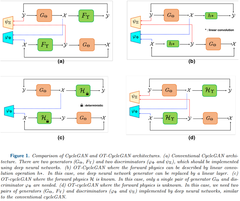
• Most important contributions of this paper: Showed that a novel cycleGAN architecture called OT-CycleGAN can be derived as a Kantorovich dual formulation if a penalized least square cost composed of physics-based data fidelity and deep learning-based inverse path penalty is used as a transportation cost.
• This is in fact a direct extension of Wasserstein-GAN(W-GAN) that was derived as a dual formulation of OT problem with Wasserstein-1 distance.
• Specifically, by additionally adding the data fidelity term, OT-cycleGAN can be derived.

Related Works

Optimal Transport (OT)

• OT provides a mathematical means to compare two probability measures.
• Formally, we say that $T:\mathcal{X}\to\mathcal{Y}$ transports the probability measure $\mu\in P(\mathcal{X})$ to another measure $\nu\in P(\mathcal{Y})$, if

\[\nu(B) = \mu(T^{-1}(B))\]

• for all $\nu$-measurable sets $B$, which is often simply represented by $\nu=T_{\sharp}\mu$, where $T_{\sharp}$ is called the push-forward operator.
• Suppose there is a cost function $c:\mathcal{X}\times\mathcal{Y}\to\mathbb{R}\cup{\infty}$ such that $c(x,y)$ represents the cost of moving one unit of mass from $x\in\mathcal{X}$ to $y\in\mathcal{Y}$.
• Monge’s original OT problem is then to find a transport map $T$ that transports $\mu$ to $\nu$ at the minimum total transportation cost:

\[\min_T\mathbb{M}(T):=\int_{\mathcal{X}}c(x,T(x))d\mu(x),\quad\text{subject to}\quad\nu=T_{\sharp}\mu\]

• The nonlinear constraint $\nu = T_{\sharp}\mu$ is difficult to handle and sometimes leads void $T$ due to assignment of indivisible mass (mass equal to zero). Kantorovich relaxed the assumption.
• Kantorovich introduced a joint measure $\pi\in P(\mathcal{X}\times \mathcal{Y})$ such that the original problem can be relaxed as

\[\min_{\pi}\int_{\mathcal{X}\times\mathcal{Y}}c(x,y)d\pi(x,y)\]

subject to

\[\pi(A\times\mathcal{Y})=\mu(A),\quad\pi(\mathcal{X}\times B)=\nu(B)\]

for all measurable sets $A\in\mathcal{X}$ and $B\in\mathcal{Y}$.

• One of the most important advantages of Kantorovich formulation is the dual formulation as stated in the folloing theorem:

• Theorem (Kantorovich duality theorem) Let $(\mathcal{X},\mu)$ and $(\mathcal{Y},\nu)$ be two Polish probability spaces (separable complete metric space) and let $c:\mathcal{X}\times\mathcal{Y}\to\mathbb{R}$ be a continous cost function, such that $

  c(x,y)

  \leq c_{\mathcal{X}}(x) + c_{\mathcal{Y}}(y)$ for some $c_{\mathcal{X}}\in L^1(\mu)$ and $c_{\mathcal{Y}}\in L^1(\nu)$, where $L^1(\mu)$ denotes a Lebesgue space with integral function with the measure $\mu$. Then, there is a duality:

\[\min_{\pi\in\Pi(\mu,\nu)}\int_{\mathcal{X}\times\mathcal{Y}}c(x,y)d\pi(x,y) = \sup_{\varphi\in L^1(\mu)}\bigg\{\int_{\mathcal{X}}\varphi(x)d\mu(x) + \int_{\mathcal{Y}}\varphi^c(y)d\nu(y)\bigg\}\\=\sup_{\psi\in L^1(\mu)}\bigg\{\int_{\mathcal{X}}\psi(x)d\mu(x) + \int_{\mathcal{Y}}\psi^c(y)d\nu(y)\bigg\}\]

where

\[\Pi(\mu,\nu) := \{\pi|\pi(A\times\mathcal{Y}) = \mu(A), \pi(\mathcal{X}\times B) = \nu(B)\}\]

and the above minimum is taken over the so-called Kantorovich potentials $\varphi$ and $\psi$, whose $c$-transforms are defined as

\[\varphi^c(y):=\inf_x(c(x,y)-\varphi(x)),\quad\psi^c(x):=\inf_y(c(x,y)-\psi(y))\]\[\min_{\pi\in\Pi(\mu,\nu)}\int_{\mathcal{X}\times\mathcal{X}}||x-y||d\pi(x,y) = \sup_{\varphi\in\text{Lip}_1(\mathcal{X})}\bigg\{\int_{\mathcal{X}}\varphi(x)d\mu(x) - \int_{\mathcal{X}}\varphi(y) d\nu(y)\bigg\}\]

PLS with Deep Learning Prior

• Example: in model based deep learning architecture (MoDL), the PLS problem is formulated as:

\[\min_xc(x;y,\Theta,\mathcal{H}) = ||y-\mathcal{H}x||^2 + \lambda||x-Q_{\Theta}(x)||^2\]

for some regularization parameter $\lambda>0$, where $Q_{\Theta}(x)$ is a pre-trained denoising CNN with the network parameter $\Theta$ and the input $x$. In this formulation, the regularization term panalizes the difference between $x$ and the “denoised” version of $x$ so that the regularization term gives high penalty when $x$ is contaminated with reconstruction artifacts.

Optimal Transport Driven CycleGAN (OT-CycleGAN)

Derivation

• OT-cycleGAN starts with a new PLS cost function with a novel deep learning prior as follows:

\[c(x,y;\Theta,\mathcal{H}) = ||y-\mathcal{H}x||^q + \lambda||G_{\Theta}(y)-x||^p\]

• Specifically, our goal is to estimate the parameter $\Theta^{\ast}$ under the unsupervised learning scenario where both $x$ and $y$ are unpaired. Since we do not have exact match between $\mathcal{X}$ and $\mathcal{Y}$ due to the unsupervised training, rather than attempting to find $x$ given $y$, we estimate joint distribution, which can considers all combinations of $x\in\mathcal{X}$ and $y\in\mathcal{Y}$. In this scenario, $x$ and $y$ can be modeled as random samples from the probability distributions on $\mathcal{X}$ and $y\in\mathcal{Y}$, respectively, but their joint probability measure $\pi(x,y)$, which we attend, is unknown.
• This is equivalent to the optimal transport problem which minimizes the average transport cost, where the average cost can be computed by

\[\mathbb{K}(\Theta,\mathcal{H}):=\min_{\pi}\int_{\mathcal{X}\times\mathcal{Y}}c(x,y;\Theta,\mathcal{H})d\pi(x,y)\]

• where the minimum is taken over all joint distributions whose marginal distributions with respect to $X$ and $Y$ are $\mu$ and $\nu$, respectively. Then, the unknown parameters for inverse problem, for example, $\mathcal{H}$ and $\Theta$ for the forward and inverse operator, respectively, can be found by minimizing $\mathbb{K}(\Theta, \mathcal{H})$ with respect to these parameters.
• This $\mathbb{K}(\Theta, \mathcal{H})$ is difficult to implement for technical issues. This is caused because it is impossible to find optimal $\pi$, as dimensionality of $\pi$ is too high.
• To address this problem, authors found its dual formulation using the Kantorovich dual formula, where the estimation of the joint distribution is not necessary. This Proposition shows that there exists interesting bounds that can be used to obtain the dual formulation.
• Proposition Consider the transportation formulation cost $\mathbb{K}(\Theta, \mathcal{H})$ of the primal OT problem using the PLS cost as mentioned above with $p=q=1$ and $\lambda=1$:

\[\mathbb{K}(\Theta,\mathcal{H})=\min_{\pi}\int_{\mathcal{X}\times\mathcal{Y}}||y-\mathcal{H}x|| + ||G_{\Theta}(y) - x||d\pi(x,y)\]

• Now let us define

\[\mathbb{D}(\Theta, \mathcal{H}) = \frac{1}{2}l_{cycle}(\Theta,\mathcal{H})+l_{OT'}(\Theta,\mathcal{H})\]

• where

\[l_{cycle}(\Theta,\mathcal{H}) = \frac{1}{2}\bigg\{\int_{\mathcal{X}}||x-G_{\Theta}(\mathcal{H}x)||d\mu(x) + \int_{\mathcal{Y}}||y-\mathcal{H}G_{\Theta}(y)||d\nu(y)\bigg\}\]

• and

\[l_{OT'}(\Theta,\mathcal{H}) = \frac{1}{2}\bigg\{\max_{\varphi}\int_{\mathcal{X}}\varphi(x)d\mu(x) - \int_{\mathcal{Y}}\varphi(G_{\Theta}(y))d\nu(y) \\+\max_{\psi}\int_{\mathcal{Y}}\psi(y)d\nu(y) - \int_{\mathcal{X}}\psi(\mathcal{H}(y))d\mu(y) \bigg\}\]

• where $\varphi, \psi$ are 1-Lipschitz functions. Then, the average transportation cost $\mathbb{K}(\Theta,\mathcal{H})$ can be approximated by $\mathbb{D}(\Theta,\mathcal{H})$ with the following error bound:

\[|\mathbb{K}(\Theta,\mathcal{H}) - \mathbb{D}(\Theta, \mathcal{H})|\leq\frac{1}{2}l_{cycle}(\Theta,\mathcal{H})\]

• Moreover, the error bound $\frac{1}{2}l_{cycle}(\Theta,\mathcal{H})$ becomes zero when $G_{\Theta}$ is an exact inverse of $\mathcal{H}$, i.e., $\mathcal{H}G_{Theta}(y) = y$ and $G_{\Theta}\mathcal{H}x = x$ for all $x\in \mathcal{X}$, $y\in\mathcal{Y}$.

• Recall that the optimal transportation map can be found by minimizing the primal OT cost function $\mathbb{K}(\Theta,\mathcal{H})$ with respect to $(\Theta,\mathcal{H})$:

\[\min_{\Theta,\mathcal{H}}\mathbb{K}(\Theta,\mathcal{H})\]

• Using Proposition, this problem can be solved by a constrained optimization problem with sufficiently small tolerance $\epsilon$ for $l_{cycle}$:

\[\min_{\Theta,\mathcal{H}}\mathcal{D}(\Theta,\mathcal{H})\quad\text{subject to}\quad l_{cycle}(\Theta,\mathcal{H})\leq\epsilon\]

• which can be solved using an unconstrained from using the Lagrangian dual:

\[\inf_{\Theta,\mathcal{H}}L(\Theta,\mathcal{H},\alpha) :=\mathcal{D}(\Theta,\mathcal{H}) + \alpha(l_{cycle}(\Theta,\mathcal{H})-\epsilon)\]

• for some $\epsilon$ dependent Lagrangian multiplier parameter $\alpha$. Therefore, the constrained optimization problem can be soved by an easier unconstrained optimization problem:

\[\min_{\Theta,\mathcal{H}}\mathbb{D}(\Theta,\mathcal{H}) + \alpha l_{cycle}(\Theta,\mathcal{H})\quad \text{or} \min_{\Theta,\mathcal{H}}l_{OT'}(\Theta,\mathcal{H}) + \gamma l_{cycle}(\Theta,\mathcal{H})\]

• where $\alpha$ or $\gamma:=\alpha + \frac{1}{2}$ is a hyperparameter to adjust during experiments.
• Finally, by implementing the Kantoronovich potential using a neural network with parameters $\Phi$ and $\Xi$, i.e., $\varphi:=\varphi_{\Phi}$ and $\psi:=\psi_{\Xi}$, we have the following cycleGAN problem:

\[\min_{\Theta,\mathcal{H}}l_{OT'}(\Theta,\mathcal{H}) + \gamma l_{cycle} (\Theta,\mathcal{H}) = \min_{\Theta,\mathcal{H}}\max_{\Phi,\Xi}l(\Theta,\mathcal{H};\Phi,\Xi)\]

• where

\[l(\Theta,\mathcal{H};\Phi,\Xi) = l_{OTDisc}(\Theta,\mathcal{H};\Phi,\Xi)+\gamma l_{cycle}(\Theta,\mathcal{H})\]

• where $l_{cycle}(\Theta,\mathcal{H})$ denotes the cycle-consistency loss and $l_{OTDisc}(\Theta,\mathcal{H};\Phi,\Xi)$ is the discriminator loss given by:

\[l_{OTDisc}(\Theta,\mathcal{H};\Phi,\Xi) = \frac{1}{2}\bigg\{\int_{\mathcal{X}}\varphi_{\Phi}(x)d\mu(x) - \int_{\mathcal{Y}}\varphi_{\Phi}(G_{\Theta}(y))d\nu(y)\\+\int_{\mathcal{Y}}\psi_{\Xi}(y)d\nu(y) - \int_{\mathcal{X}}\psi_{\Xi}(\mathcal{H}x)d\mu(x)\bigg\}\]

• Note that the Kantoronovich dual problems should be maximized with respect to 1-Lipschitz functions, so the paremeterized functions $\varphi$ and $\psi$ should have sufficiently large capacity to approximate any 1-Lipschitz function. This is why authors employ deep neural network to model the 1-Lipschitz Kantoronovich potentials. These $\varphi:=\varphi_{\Phi}$ and $\psi :=\psi_{\Xi}$ correspond to the W-GAN discriminators.
• Specifically, $\varphi_{\Phi}$ tries to find the difference between the true image $x$ and the generated image $G_{\Theta}(y)$, whereas $\psi := \psi_{\Xi}$ attempts to find the fake measurement data that are generated by the synthetic measurement procedure $\mathcal{H}x$

Implementation

• We only consider $p=q=1$ due the inequalities and for 1-Lipschitz $\varphi$ and $\psi$.
• Imposing 1-Lipschitz condition for the discriminator is the main idea of the Kantoronovich dual formulation as W-GAN. Therefore, care should be taken to ensure that the Kantoronovich potential becomes 1-Lipschitz.
• In this paper, authors used WGAN with the gradient penalty (WGAN-GP), where the gradient of the Kantoronovich potential is constrained to be 1.
• Specifically, for

\[l_{cycle} = \int_{\mathcal{X}}||x-G_{\Theta}(\mathcal{H}x)||d\mu(x) + \int_{\mathcal{Y}}||y-\mathcal{H}G_{\Theta}(y)||d\nu(y)\]

and

\[l_{Disc}\text{ or the }l_{OTDisc} = \int_{\mathcal{X}}\varphi_{\Phi}(x)d\mu(x) - \int_{\mathcal{Y}}\varphi_{\Phi}(G_{\Theta}(y))d\nu(y)\]

we get

\[l_{OTDisc}(\Theta,\Phi) = \bigg(\int_{\mathcal{X}}\varphi_{\Phi}(x)d\mu(x) - \int_{\mathcal{Y}}\varphi_{\Phi}(G_{\Theta}(y))d\nu(y)\bigg)\\-\eta\int_{\mathcal{X}}(||\nabla_{\tilde{x}}\varphi_{\Phi}(x)||_2-1)^2d\mu(x)\]

where $\eta>0$ is the regularization parameters to impose 1-Lipschitz property for the discriminators, and $\tilde{x} = \alpha x + (1-\alpha)G_{\Theta}(y)$ with $\alpha$ being random variables from the uniform distribution between $[0,1]$